


Neural Operators
Joseph Fourier
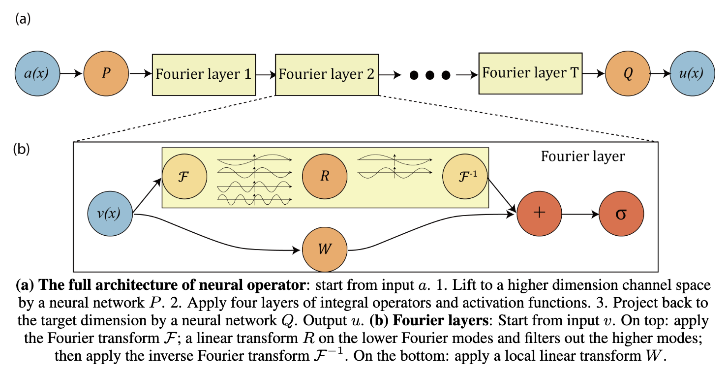
A screenshot from the FNO paper.
This post is based on a tweet thread I’d written earlier,
Fourier Neural Operators. I steel myself whenever jumping into the frequency domain 🫨. Little late, but finally got around to studying them! Based on this very clearly written paper by @zongyili_nyu. I recommend you read it yourself! 🧵1/8 👇https://t.co/ONekJAlow6 pic.twitter.com/tw2Hqp1JXD
— Ibrahim (@hazrmard) August 4, 2026
Fourier Neural Operators
Let’s start with Fourier Neural Operators (FNOs). I steel myself whenever jumping into the frequency domain 🫨. Finally got around to studying them! Based on this very clearly written paper by Zongyi Li. I recommend you read it yourself!
https://arxiv.org/pdf/2010.08895
The big problem in the big domain: using neural networks for physics simulations has seen quite some work (see PINNs, NeuralODEs). Problem? The output is baked in. If you trained a sim on a 100x100x100 grid, that’s all you’ll ever see. Cannot zoom in, unless you train on a finer grid. This is where a couple of insights into frequency domain come in. First, an aside on how sims work:
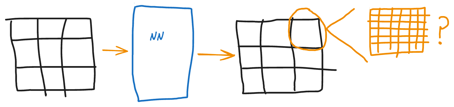
A NN can be trained on a certain grid of inputs. But can the NN generalize to arbitrarily fine grids? A grid can be along space or time dimensions.
Physics sims solve partial differential equations. Let’s say we’re looking at n-body problems. The bodies have some spatial distribution. The equation is $a=F/m$, where $F$ is the gravitational force from all the bodies in the sim. The change in position may be due to the body x itself i.e. own thrust (local) and due to bodies y all over the sim space (global). We need to account for the effects of both. So, $a=F/m$ is solved for each point in the sim, and each point in the sim looks at every other point. This operation is called convolution. The sim step for each point x looks like:
$$ \frac{dx}{dt}=(W(x)+b) + \int K(x, y)v(y) dy, $$
where $K$ is the gravitational field of y at x, and $v(y)$ is a representation of point y (here, y’s mass). $Wx+b$ is local change due to x itself. It only depends on x. $\int K(x, y)v(y) dy$ is global. It depends on all points y in the sim space. Complexity when repeated for all x? O($n^2$). Back to frequency insights:
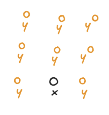
The simulation of a point x depends on its own (local) state, and the effects of neighbouring (global) states.
A wave with a frequency f has infinite resolution. It’s just a function (e.g $\sin(2 \pi f\cdot t)$) - you can keep zooming in.
(Periodic) Functions in space can be represented as superpositions of various frequencies i.e. a list of coefficients in freq domain.
Convolution in frequency domain is a point-wise multiplication, instead of integration i.e. $O(N^2)\rightarrow O(N)$.
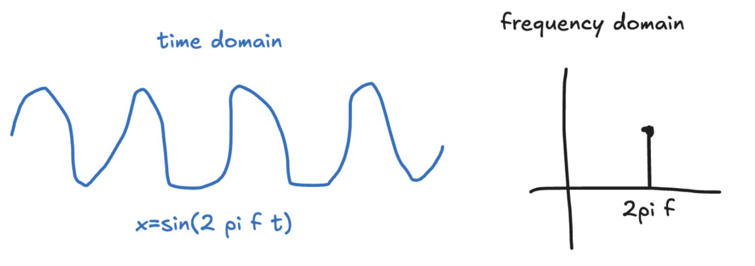
Time/frequency domains are complementary. An infinitely long wave of a single frequency in time becomes a point in frequency domain. Conversely (not shown), an infinitely large combination of frequencies can represent a a single point in time domain.
What if: we convert the inputs into frequency domain, convolve them, and convert back into space domain? (Fast) Fourier transform is $O(NlogN)$, multiplication is $O(N)$. Therefore total complexity is $O(NlogN)$, and we get infinite resolution! This is a Fourier Neural Operator. A NN layer that handles frequency conversion, convolution, and conversion back to space.
Now, the nitty-gritty caveats & observations:
frequency domain assumes periodic boundary conditions (e.g. sine wave repeats every $2 \pi$).
physical systems are non-linear.
local effects are represented by higher frequencies, global by lower frequencies. We can fix this by bifurcating across space / frequency domains:
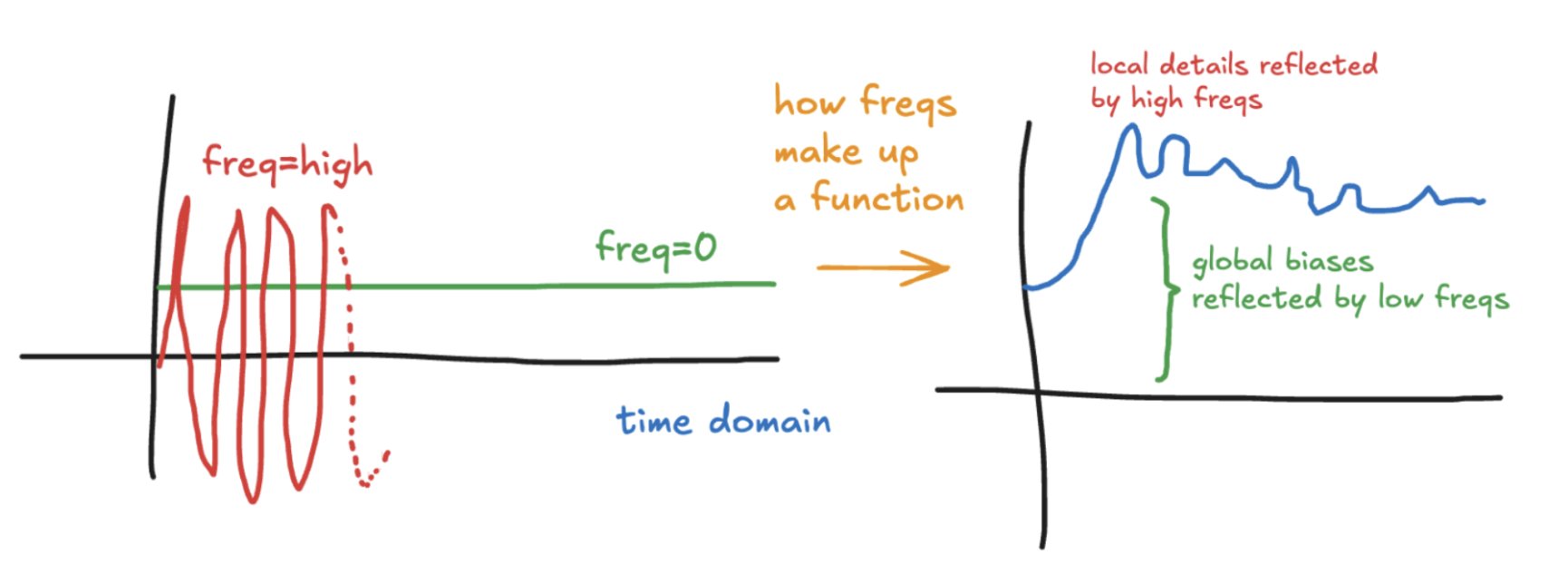
Lower frequencies show up as global biases, and higher frequencies show up as local effects.
A FNO layer ends with an activation function σ. The activation function accumulates spatial and frequency processing of inputs: σ(W x + b + 𝓕^-1(𝓕(K)*𝓕(x))). The frequency stream zeroes out higher frequencies in the frequency domain, applies some linear transformation 𝓕(K), and converts back to the spatial domain. Translation: integrating global effects. The spatial stream applies a linear transformation W to points. Translation: local effects. The activation, along with W, re-introduces non-linearities & higher freqs in the output such as boundary conditions omitted in the freq domain.
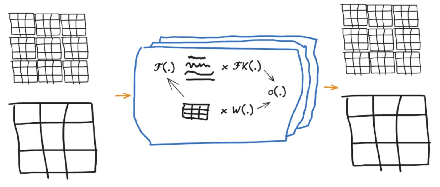
A FNO layer concurrently solves the input grid in time and frequency domain. In time domain, it applies local effects. In frequency domain, higher frequencies are suppressed, and the global effects (lower frequencies) are processed. Finally, an inverse fourier transform brings the concurrent streams back together in time domain, where an activation function (non-linearity) helps represent non-linear boundary conditions.
We can pass finer grids. The spatial part is a pointwise transform and the frequency transform doesn’t care about space. The same learned weights work out of the box.
Cons: needs high quality data, uniform grids. Pros: fast, resolution invariant.
The following widget shows how a 1D differential equation solution can be modelled efficiently by delegating some of the learning to frequency domain. Play around with the knobs and sliders. Look out for the mean squared error (MSE) between a FNO model and a vanilla Multi Layer Perceptron (MLP). You can single out the prediction of different parts of the FNO model. For example, the frequency branch shows how coefficients for lower modes are learned, whereas higher frequencies are suppressed.
Extending Neural operators to other bases
After my FNO shallowdive, I had an epiphany: I could replace Fourier basis with wavelets for better localizability. Even better! I could have learnable Koglomorov Arnold basis to tailor to diverse domains.
It’s been done already!
A note on “5 trillion context”
I wrote the thread a little before the launch of a startup (Accelerated Understanding) by one of the co-authors of the FNO paper, Dr. Anima Anandkumar. The marketing copy stated their models were capabie of a trillion token context window. In this age of LLMs, “token” has become a load-bearing accounting term for the size of inputs chat models can handle. I hope this article makes it clear that comparing a token to a point in a grid representing a physical phenomenon is an apples-to-oranges comparison.
A point grid =/= context especially in the realm of frequency domain. I get the sales aspect of calling it context, given hot how LLMs are. Technically, one can have infinitely fine grid represented finitely in freq domain, and claim an infinite context.
— Ibrahim (@hazrmard) September 4, 2026