Modern control: Solutions & state transition matrices
Section: Home / Post / Control systems
Categories: Engineering,
Tags: Matlab, Control Systems,
The state equation for a linear time-invariant system:
$$ x’(t) = A x(t) + B u(t) $$
Can be solved for $x(t)$. We collect all terms in $x$:
$$ x’(t) - A x(t) = B u(t) $$
Multiply equation by $e^{-At}$
$$ x’(t) e^{-At} - A x(t) e^{-At} = B u(t) e^{-At} $$
Using product rule $d(f;g) = f;dg + g;df$, where:
To give:
$$ \frac{d}{dt} (e^{-At} x(t)) = B u(t) e^{-At} $$
Which can be integrated on the limits $t = t_0 \rightarrow t$:
The solution to the state equation is:
This can be plugged into the output equation to compute system outputs.
State transition matrix
The term $e^{At}$ is called the state transition matrix. It is an exponental of the system matrix which relates the change in state to the current state. The exponential can be calculated in several ways through Taylor series expansion an inverse laplace transform, spectral decomposition, or the Cayley-Hamilton theorem.
In MatLab:
| |
For the case of time-varying systems, the state transition matrix is not a simple exponential but a function $\phi(t, t_0)$ unique to the system. The general solution of the state equation for time-varying systems becomes:
More details on the general solution can be found in the WikiBook.
Example - spring mass system
Using the matrices found in the last post, we have the state space matrices:
Making some assumptions for the constants, we can define the matrices in MatLab:
| |
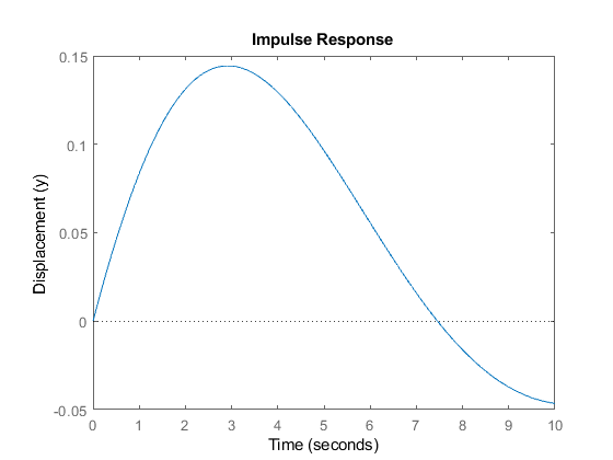
Impulse response
Using the matlab command, we get:
| |

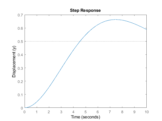
Impulse response
Using the matlab command, we get:
| |
