Modern control: State space equations

Monday, Sep 24, 2018
Section: Home / Post / Control systems
Categories: Engineering,
Tags: Matlab, Control Systems,

In modern control approaches, systems are analyzed in time domain as a set of differential equations. Higher order differential equations are decomposed into sets of first order equations of state variables that represent the system internally. This produces three sets of variables:

Input variables are stimuli given to the system. Denoted by $u$.
Output variables are the result of the current system state and inputs. Denoted by $y$.
State variables represent the internal state of a system which may be obscured in the output variables. Denoted by $x$.

State-space equations

A state-space model is represented by two sets of equations.

State equation

The state equation represents how the internal state of the system is changing with time. The rate of change of state depends on the current state, inputs, and time.

$$ x’(t) = f(t, x(t), u(t)) $$

Where $x$ is a vector of state variables. For the case where $x’(t)$ is a linear combination of inputs and states, and the system is time invariant:

$$ x’(t) = Ax(t) + Bu(t) $$

Output equation

The output equation represents what will be observed from the system in response to the inputs. The outputs also depend on the current state, inputs, and time.

$$ y(t) = g(t, x(t), u(t)) $$

And for the linear, time invariant case:

$$ y(t) = Cx(t) + Du(t) $$

State-space matrices

Each matrix $A, B, C, D$ has a special meaning regarding the behaviour of the system.

$A$ - System matrix: $A$ provides the rate of change of state from the current system state.
$B$ - control matrix: $B$ provides the rate of change of state from the control input.
$C$ - output matrix: $C$ calculates the contribution of the system state to the system output variables.
$D$ - feed-forward matrix: $D$ calculates the contribution of the control input to the system output variables.

Example - spring mass system

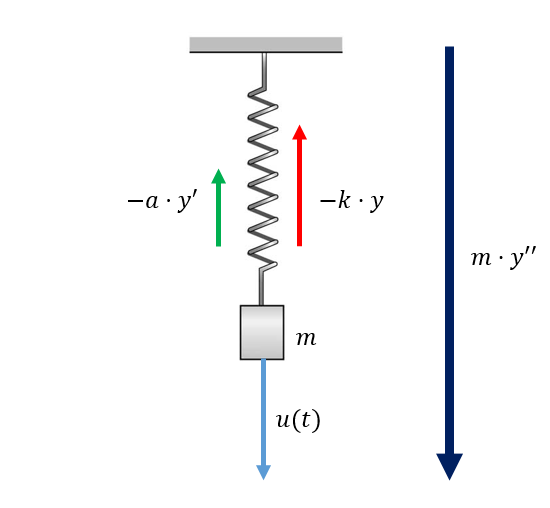
A spring mass system showing the 3 acting forces and the resultant force.

Let’s take a spring mass system. There are three forces acting on it:

$u(t)$ - the external input force acting on the mass.
$-k \cdot y(t)$ - The force due to the spring. The force acts in the direction opposite to the extension/compression of the spring. It is proportional to the amount of extension/compression.
$-a \cdot y’(t)$ - The viscous force i.e. air resistance. The force acts in the direction opposite to the motion of the mass. It is proportional to the velocity of the mass.

Summing all components up gives the resultant force, according to Newton’s second law of motion:

$$ \begin{align*} m \cdot y''(t) &= u(t) - k \cdot y(t) - a \cdot y'(t) \\ m \cdot y''(t) + k \cdot y(t) + a \cdot y'(t) &= u(t) \end{align*} $$

This is a second order ordinary differential equation (ODE). It relates the output variable $y$ (the displacement of the mass) to the input variable $u$ (the external force). The equation can be broken down into two first order differential equations by appointing $n$ state variables for an $n^{th}$ order ODE for the $0^{th}$ through $(n-1)^{th}$ derivatives of the output variable.

$$ \begin{align*} x(t) = \begin{bmatrix} x_1(t) \\ x_2(t) \\ \end{bmatrix} = \begin{bmatrix} y(t) \\ y'(t) \\ \end{bmatrix} \end{align*} $$

Then differentiating and substituting for state variables.

$$ \begin{align*} x'(t) &= \begin{bmatrix} x_1'(t) \\ x_2'(t) \\ \end{bmatrix} = \begin{bmatrix} x_2(t) \\ y''(t) \\ \end{bmatrix} \\ x'(t) &= \begin{bmatrix} x_2(t) \\ \frac{1}{m}(u(t) - k \cdot x_1(t) - a \cdot x_2(t)) \\ \end{bmatrix} \\ x'(t) &= \begin{bmatrix} x_2(t) \\ \frac{1}{m}(- k \cdot x_1(t) - a \cdot x_2(t)) \end{bmatrix} + \begin{bmatrix} 0 \\ \frac{1}{m}u(t) \end{bmatrix} \\ x'(t) &= \begin{bmatrix} 0 & 1 \\ \frac{-k}{m} & \frac{-a}{m} \end{bmatrix} \cdot x(t) + \begin{bmatrix} 0 \\ \frac{1}{m} \end{bmatrix} \cdot u(t) \end{align*} $$

Which gives us for the state equation:

$$ \begin{align*} A = \begin{bmatrix} 0 & 1 \\ \frac{-k}{m} & \frac{-a}{m} \end{bmatrix}, B = \begin{bmatrix} 0 \\ \frac{1}{m} \end{bmatrix} \end{align*} $$

Similarly, knowing that $x_1(t) = y(t)$, we can construct:

$$ \begin{align*} y(t) = \begin{bmatrix} 1 & 0 \end{bmatrix} \cdot x(t) + \begin{bmatrix} 0 \end{bmatrix} \cdot u(t) \end{align*} $$

Which gives us for the output equation:

$$ C = \begin{bmatrix} 1 & 0 \end{bmatrix}, D = \begin{bmatrix} 0 \end{bmatrix} $$