


A Poor Man's Introduction to Reinforcement Learning
Section: Home / Post
Categories: Engineering,
Tags: Artificial Intelligence, Reinforcement Learning,
Reinforcement Learning (RL) is one of the many ways to implement artificial intelligence (AI). AI is the design of “intelligent” agents that maximize their chances of success at some goal. The goal can belong to any problem: from winning a game of tic-tac-toe, to recognizing speech, to steering a car.
A problem can be approached in many different ways. An agent can search for all possible options and choose the best. Or the problem can be formulated as a set of logical rules which the agent then applies at each step. The former way may require searching too many options. The latter may require meticulous representation of the nuances in a system.
RL is built on experience. With each action an agent takes, it gets some feedback - reinforcement - from its environment. It uses that reinforcement to get better. So RL agents start off poorly, with the expectation that they will get better as they blunder their way through the problem.

Let’s see what sticks: an illustration of various approaches towards implementing AI. Left: An agent tries all options. Centre: An agent formulates the problem and derives the best choice. Right: An agent learns from experience (reinforcement).
A reinforcement learning problem can be viewed as repeated interactions between the agent and the environment. An agent can be in one of a number of states. At every instance, an agent has a set of actions it can take. For each action, the agent will transition to another state. Also, for each action the agent will get some feedback from the environment.
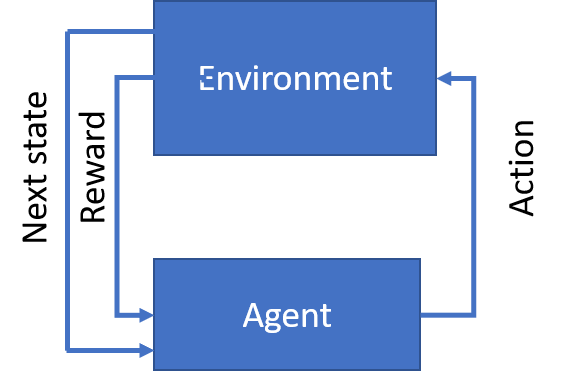
The goal of an agent is to maximize the reward it gets from the environment. To do that, it learns the value of each state from experience. The value of a state is the maximum total reward the agent can expect in the future if it goes to that state. The agent explores the environment and takes a record of the rewards it received. Once values of states are sufficiently learned, an agent can exploit them by acting towards the most valuable state at each step.
The value of a state is the maximum total reward the agent can expect in the future if it goes to that state.
The life of an agent, therefore, is split into two parts: exploraton and exploitation. During exploration, the agent may forego valuable states to take random/unrewarding actions. Perhaps they may lead to even greater rewards. During exploitation, an agent relies on previously learned values for its choice of actions. How an agent chooses actions is known as its policy. It can be based on a single rule (take most rewarding action), or it can change over time, or it can be different for exploration and exploitation.
The policy of an agent is the set of rules which govern the choice of the next action from the agent’s current state.
How are the values of states calculated? To rephrase the definition of value: it is the total reward from the most rewarding combination of actions from a state. For each state, an ideal agent will chart all possible trajectories of actions into the future. It will explore each of those trajectories and note the highest reward which will become the value.
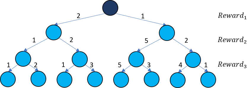
An agent charts all possible action trajectories from the current state (dark blue) to find the most rewarding combinaton of actions. The total reward of that combination is the state’s value. In this case the most rewarding combination is from rewards 1-5-5 which gives a value of 11.
Dynamic Programming
Sounds daunting, no? The problem can be rephrased using a dynamic programming approach. Dynamic programming breaks a problem down into similar and smaller problems. Each of those problems are recursively broken down into smaller versions of themselves until the simplest problem is reached for which we know the answer. We can then “rebuild” our solution from the bottom up.
In the illustration, the agent has a lifetime of 3 steps. At each step, it can take 2 actions, and therefore earn 2 rewards. This gives us 8 possible action trajectories or reward combinations. The value of the current state, $s0$, is the maximum attainable reward:
$$ value(s0) = \max_{actions}(Reward_{1} + Reward_{2} + Reward_{3}) $$
We can observe that the maximum reward is the maximizing combination of the immediate reward from the current state, and the following rewards from the next state:
$$ value(s0) = \max_{actions}(Reward_{1} + \max_{actions}(Reward_{2} + Reward_{3})) $$
The intuition behind this is simple: for a set of all 3 actions to have optimal rewards, the subset of the last 2 actions must necessarily be optimal too.
Notice we have decomposed our maximization problem into a smaller, similar problem. By the definition of value:
$$value(s0) = \max_{actions}(Reward_{1} + value(s1))$$ $$value(s1) = \max_{actions}(Reward_{2} + value(s2))$$ $$\vdots$$
Where $s1$ is the state that follows $Reward_{1}$. This is known as the Bellman Equation. The value of a state depends on the value of neighbouring states. So the agent first solves for those values. Then it compares them to find the best combination for the current value.

Dynamic programming looks at all reachable states to calculate the value of the current state.
The dynamic approach is thorough: it looks at every single state to find value. This presents a problem, however: what if there are too many states? What if the environment is continuous and there are infinitely many states? What if the agent needs to learn before a deadline? The methods that follow are faster, but they approximate the true value of states.
Monte Carlo methods
Enter: Monte Carlo methods. Monte Carlo methods forego a complete traversal of state-space in favour of sparser, episodic sampling. The learning process of an agent is comprised of multiple episodes. For each episode, the agent starts at some state. It does not look at all neighbouring states, but picks one action to go to the next state. At each step, the agent makes a choice of action until it reaches a terminal state. This concludes the episode. An episode is a single trajectory of actions. The agent keeps a record of states it encounters in an episode, and the rewards it gets from actions. For each state, the return is the sum of all rewards that follow.
The return of a state is the total reward that follows from that state based on the agent’s action selection policy.
Over multiple episodes, an agent may see a state many times. Each time, an agent calculates the return for that state. The average return is the total reward an agent can expect from that state. An agent approximates the value of a state by its average return. If the agent’s policy (how it chooses actions) is somewhat greedy i.e. it prefers states with higher returns, then over time the value approximation will get closer to the true value of states.
$$value(s0) = Average(Reward_{1} + Reward_{2} + \ldots) = Average(return(s0))$$ $$value(s1) = Average(Reward_{2} + Reward_{3} + \ldots) = Average(return(s1))$$ $$\vdots$$
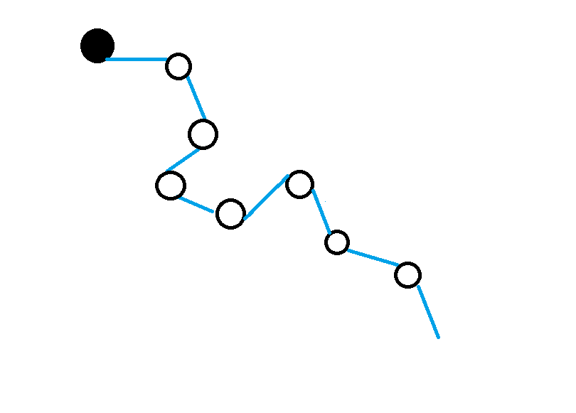
Monte Carlo approaches approximate value of states from average returns over multiple episodes. This illustration shows a single episode. Episodes may cirsscross over state space, so each state is sampled multiple times.
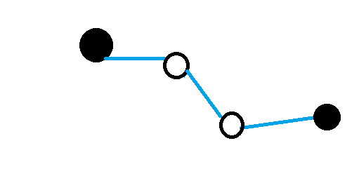
Monte Carlo methods are appropriate where a learning task can be broken up into episodes. For example a game of tic-tac-toe, chess, or go where an episode ends when one side wins. Monte Carlo methods update value estimates after each episode ends. But what if there is no end? What if episodes are too long?
Temporal Difference Learning
Temporal Difference methods alleviate this problem. Like Monte Carlo approaches, they are episodic, and require a policy for exploration. Similarly, they approximate the value from average returns of a state. Unlike Monte Carlo methods, they update value estimates after each action. Let’s say an agent is at a state $s0$, and takes an action towards $s1$ to get a reward $Reward_{1}$. We know that the return of $s0$ is the sum of all future rewards on that policy:
$$return(s0) = Reward_{1} + Reward_{2} + \ldots$$
The agent has not yet seen $(Reward_{2} + \ldots)$. That is the return of the next state, $s1$. We can substitute the average return of the next state instead. That is just our current estimate of the value of $s1$!
$$return(s0) = Reward_{1} + Average(return(s1)) = Reward_{1} + value(s1)$$
Herein lies the difference with Monte Carlo methods: instead of explicitly calculating the return, we estimate it by observing the immediate reward and backing-up the remainder from the agent’s previous experience. Since we introduced one new piece of information - $Reward_{1}$ - our new estimate of the return of $s0$ is an updated approximation of the value of $s0$. The error with respect to current value approximation is:
$$ error(s0) = return(s0) - value(s0) $$
The current $value(s0)$ needs to be changed by $error(s0)$ to get the next approximation. However we do not want to update it all at once. Perhaps the agent chose a bad action which gave a poor return. So we weigh the error by a learning rate $\alpha$ to update value:
$$ value(s0) = value(s0) + \alpha \times error(s0) $$
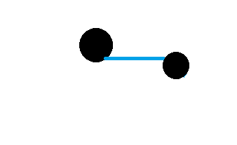
Temporal Difference methods update the value of states after a single step. They use the immediate reward and back-ups of previously calculated values to calculate the change.
At each step, the agent observes the reward, calculates a new estimate of return from the previously calculated values, and updates the value of the current state. With each iteration, given a partially greedy policy, the agent can expect to get better approximations of the true value of states.
A compromise between Monte Carlo and Temporal Difference methods are the Temporal Difference($\lambda$) methods. Instead of using the immediate reward and back-ups of values to estimate return, they observe rewards for an additional $\lambda$-steps before taking backups:
$$ return(s0) = Reward_{1} + \ldots + Reward_{\lambda + 1} + value(s\lambda + 1) $$
When $\lambda=0$, this decays into the simple Temporal Difference approach. When $\lambda=\infty$, it becomes a Monte Carlo approach.
Temporal Difference($\lambda$) methods update the value of states after multiple steps. They use future rewards and back-ups of previously calculated values to calculate the change.
So far, the agent’s exploration has been very linear. It picks one action at each state without considering the influence of neighbouring states. The n-step Tree Backup approach is a generalization of temporal difference methods. When calculating the return, the agent also backs up values of states from actions not taken. This means that the return of a state is now more representative of the average return because the agent considers multiple actions.
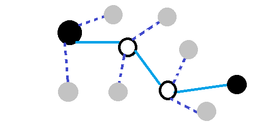
n-Step Tree Backup approaches weigh the rewards of actions taken, and the values of reachable states not traversed.
A mathematical formulation for the n-Step Tree Backup return would be too math-y for the purposes of this article. Resources to a more rigorous discussion of these concepts are included at the end.
A Final Word
The approaches discussed so far all fall under value iteration. An agent calculates the values of states. Whenever an action needs to be chosen, the current value function is used to find an appropriate action. The agent generates new episodes and values until the values converge.
In Policy iteration, the agent defines its policy and uses it to generate episodes and values until the values do not change. Then it re-calculates a new policy and repeats the process until the policy converges.
The following illustration gives an overview of the methods discussed here. It by no means is an exhaustive summary of reinforcement learning theory. It shows the different ways agents explore state space to come to a decision about the best actions to take.
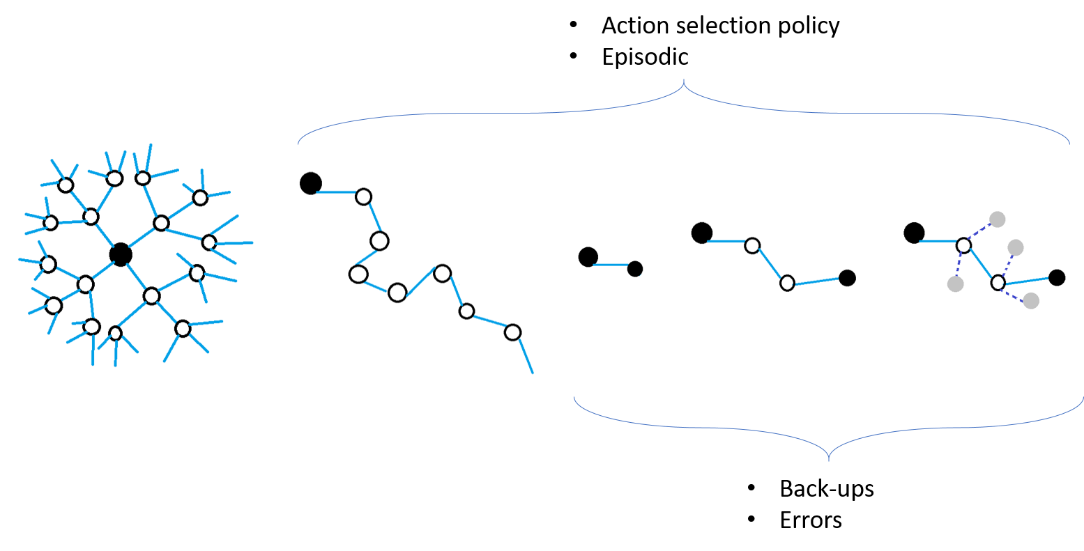
Reinforcement learning methods can derive agent behaviour from dense and sparse sampling of state space.